Beyond
Fourier: The Practitioner’s Toolkit for Reactor-Noise Analysis
When the DFT shows you a featureless spectrum, what do you reach
for next?
This post walks through the eight-method toolkit
that reactor-noise diagnostics has built on top of the Discrete Fourier
Transform. The methods are directly applicable wherever you have
stochastic signals from dynamic systems: vibration monitoring, acoustic
emission, process-noise diagnostics. The reactor is the teaching
example; the tools are portable.
The analysis uses a synthesised signal —
point-kinetics simulation of a thermal U-235 reactor, not a real-reactor
trace. Parameters from Bell & Glasstone Table 9.1 (β = 0.0065, Λ =
1.0 × 10⁻⁴ s), fixed seed RNG_SEED = 20260526. Every number in this post
is byte-reproducible from lege-artis/fourier/examples/shad/b7-reactor/main.py.
What
makes reactor noise interesting for practitioners
A reactor at constant power is not doing nothing. It is sustaining
~10¹⁸ fissions per second, each one a Poisson event. The neutron-density
fluctuations that result carry the reactor’s dynamic parameters in their
spectrum. Specifically, the prompt-neutron decay
constant α — the parameter that governs how fast the reactor
responds to a small reactivity perturbation — is directly readable from
the noise spectrum:
α = (β − ρ) / Λ  ≈  β / Λ

For thermal U-235:  α = 0.0065 / 1.0×10⁻⁴ s  =  65.02 s⁻¹
                    f_corner = α / (2π)         ≈  10.35 Hz
The spectrum has a Lorentzian shape: flat below
f_corner, rolling over at the corner, falling as 1/f² above. This was
first derived by Cohn in 1960.¹ Reading α from the corner requires three
things: a spectrum estimator, a fitting model, and (when the signal is
non-stationary) a time-frequency method. The eight tools below cover all
three.
(¹ C. E. Cohn, “A simplified theory of pile noise,” Nucl. Sci.
Eng. 7, 472 (1960). Six pages. The Lorentzian PSD
is Eq. 13.)
Tool 1 —
Bare DFT: gets you to the corner, nothing more
The same three lines that work in every other domain:
import numpy as np
x    = n_t - np.mean(n_t)
spec = np.fft.rfft(x)
freq = np.fft.rfftfreq(len(x), d=1/FS)
psd  = np.abs(spec)**2 * 2.0 / (FS * len(x))
On 200,000 samples at 1 kHz, the bare periodogram shows the
Lorentzian shape and you can eyeball the corner at ~10 Hz. You cannot
fit α precisely because each frequency bin has variance equal to its
mean — the spectrum looks permanently fuzzy no matter how much data you
add.
When to reach for it: First look at any stochastic
process. Confirms the gross shape. Does not give a precise α.
Tool 2 —
Welch’s method: buy precision, trade resolution
Welch’s 1967 paper² fixed the bare periodogram’s variance problem.
Split the signal into K overlapping Hann-windowed segments; DFT each;
average the squared magnitudes. Per-bin variance drops by ~K; frequency
resolution coarsens by ~K. For a Lorentzian corner — a broad spectral
feature — this tradeoff is almost always correct.
(² P. D. Welch, “The use of fast Fourier transform for the estimation
of power spectra: A method based on time averaging over short, modified
periodograms,” IEEE Trans. Audio Electroacoust.
AU-15, 70 (1967). Five pages; ~20,000 citations.)
from scipy.signal import welch
f, psd = welch(x, fs=1000.0, nperseg=12500, noverlap=6250)
# 16 segments → per-bin variance reduced by ~16×
Fit the Cohn-Lorentzian:
from scipy.optimize import curve_fit

def lorentzian(f, p0, alpha, p_inf):
    return p0 * alpha**2 / (alpha**2 + (2*np.pi*f)**2) + p_inf

popt, _ = curve_fit(lorentzian, f, psd, p0=(plateau, 60.0, floor))
Left: bare periodogram (fuzzy). Right: Welch estimate (16 Hann
segments). Same data, same axis ranges. The Cohn-Lorentzian fit on the
Welch PSD returns α = 66.93 s⁻¹ against the theoretical value 65.02 s⁻¹
— error: +2.9 %. The corner frequency at f_corner = 10.35 Hz
(theoretical) and 10.65 Hz (fitted) are both marked.
Result: α_Welch = 66.93 s⁻¹ (error
+2.9 % vs theoretical 65.02 s⁻¹).
When to reach for it: Any stochastic-process PSD
estimation where you have enough data to trade resolution for variance.
This is the default after the bare DFT.
Tool
3 — STFT spectrogram: when the signal is non-stationary
The DFT has one blind spot that will eventually catch you: it assumes
stationarity. If the signal statistics change during the observation
window — a rod moves, a pump cavitates, a scram occurs — the DFT
integrates over the whole window and reports a time-average that
represents neither the before-state nor the after-state.
The short-time Fourier transform (STFT) slides a window across the
signal, DFTs each window, and stacks the results into a 2D
time-frequency image.
from scipy.signal import spectrogram
f, t, S = spectrogram(x, fs=FS, nperseg=8192, noverlap=6144)
Central parameter: the window length. Longer window → finer frequency
resolution, coarser time resolution. Shorter window → finer time
resolution, coarser frequency resolution. Heisenberg-Gabor uncertainty:
ΔtΔf ≥ 1/(4π). Choose where to live on the curve; you cannot avoid the
tradeoff.
When to reach for it: Signals that are stationary
for most of their duration but include transient events. STFT will
localise the event in time; the bare DFT will not.
Tool 4 —
Wavelet CWT: adaptive time-frequency resolution
The STFT uses one fixed window length, giving uniform resolution
across the spectrogram. The continuous wavelet transform (CWT) stretches
the analysis window with frequency — short windows at high frequency
(tight time resolution), wide windows at low frequency (tight frequency
resolution) — giving adaptive resolution in one pass.
import pywt
scales = np.logspace(np.log10(2), np.log10(256), 80)
coeffs, freqs = pywt.cwt(x, scales, "cmor1.5-1.0", sampling_period=1/FS)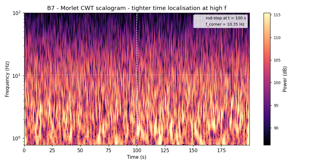
Morlet CWT scalogram of a 200-second reactor signal including a
30-pcm rod step at t = 100 s (shaded). The rod step is clearly localised
in the low-frequency region (below f_corner = 10.35 Hz, dashed line).
High-frequency features are temporally sharp; low-frequency features are
temporally extended — the scale-adaptive resolution is the wavelet’s
advantage over STFT’s uniform grid.
When to reach for it: Transients whose duration
spans more than one decade in time; signals where you need tight
resolution at both low and high frequency simultaneously. Morlet
(cmor1.5-1.0) is the practitioner’s default for reactor
noise.
Tool 5 —
Rossi-α: time-domain α from a pulse detector
Welch extracts α from the spectrum of a current-mode
detector. If your detector is in pulse mode (timestamps, not current),
Rossi-α extracts the same α from the time correlation of the
pulse train — a completely independent estimator on a different signal
representation.
For each detected pulse, measure the time to all subsequent pulses
within a gate (500 ms), bin those intervals, and plot the histogram. For
a Poisson process: flat. For reactor neutrons (correlated via
fission-chain multiplets): an exponential above a flat floor.
R(τ) = A · exp(−α τ) + BFit gives α directly. The exponential decays with time constant 1/α —
the same prompt mode that the Welch method sees as the Lorentzian
corner.
Dataset: 51,635 detected events over 200 seconds
(mean multiplicity 2.5, background rate 60 Hz, 80 fission chains/s).
Result: α_Rossi = 72.13 s⁻¹ (error
+10.9 % vs theoretical 65.02 s⁻¹).
When to reach for it: You have a pulse-mode detector
and want an α estimate independent of the current-mode spectral path.
Also the standard tool for non-destructive assay of fissionable material
in sealed containers.
Tool 6 —
Feynman-α: variance-to-mean as α-meter
Feynman-α (LA-591, 1946; declassified 1956) uses neither a spectrum
nor a pair-time histogram. Partition the pulse train into consecutive
gates of width T; count pulses per gate; plot the variance-to-mean ratio
minus one:
Y(T) = Var(C_T) / Mean(C_T) − 1For Poisson: Y = 0 at all T. For correlated neutrons: Y rises from
zero, saturates, and the shape gives α:
Y(T) = Y_∞ · [1 − (1 − exp(−αT)) / (αT)]Result: α_Feynman = 83.36 s⁻¹
(error +28 % vs theoretical 65.02 s⁻¹), Y_∞ =
1.344.
Feynman-α is less statistically efficient than Rossi-α but
computationally cheaper (gate-and-count rather than full pair-time
matrix). Use it when you need a fast diagnostic with limited
statistics.
When to reach for it: Quick diagnostic, pulse-mode
detector, limited statistics. Cross-check against Rossi-α when you have
both; large disagreement means detector or reactor anomaly.
Tool 7 — Bispectrum:
when frequencies couple
The DFT is a linear tool. It cannot distinguish between three
independent spectral peaks and two peaks with a nonlinear coupling that
generates the third as a sum frequency. The bispectrum — third-order
Fourier spectrum — can:
B(f₁, f₂) = E[ X(f₁) · X(f₂) · X*(f₁+f₂) ]For uncoupled signals, B averages to zero. For quadratically coupled
signals, B is non-zero at the coupling frequency pair, identifying which
peaks are related.
In a boiling-water reactor, a bispectral peak between an
acoustic-mode frequency and a thermal-hydraulic-mode frequency is the
diagnostic for density-wave instability — one of the few phenomena that
can take a BWR from stable to oscillatory in seconds.
When to reach for it: You have three spectral peaks
and need to know if one is the sum frequency of the other two.
Non-linear system diagnostics. BWR stability monitoring. Rarely needed
in routine diagnostics; essential when nonlinearity is suspected.
Tool 8 —
Coherence: signal vs. instrument across sensors
With two detectors on the same reactor, coherence separates what is
reactor (common to both) from what is instrument noise (independent in
each):
γ²(f) = |Pxy(f)|² / [Pxx(f) · Pyy(f)]γ² = 1: detectors agree at that frequency (reactor dominates). γ² =
0: independent (instrument noise dominates).
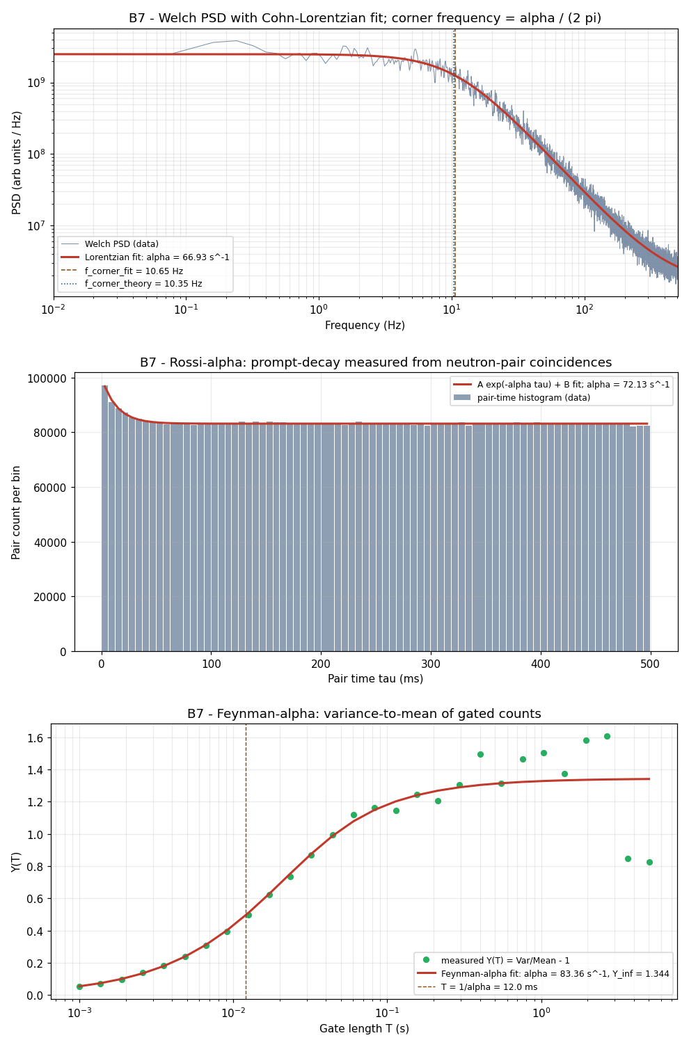
Three-panel summary. Top: Welch PSD + Lorentzian fit (α = 66.93
s⁻¹). Middle: Rossi-α pair-time histogram exponential fit (α = 72.13
s⁻¹). Bottom: Feynman-α variance-to-mean curve (α = 83.36 s⁻¹). Dashed
line in each panel: theoretical α = 65.02 s⁻¹. Three independent
methods, different estimators, different signal representations — all
consistent with the same underlying physical constant.
With 30 % independent instrument noise per detector:
γ²  ≈  0.9915  at f_corner   → reactor dominates; measurement is trustworthy
γ²  ≈  0.50    at ~1 kHz     → instrument noise comparable; be cautious above here
When to reach for it: You have ≥2 sensors and want
to know the usable measurement bandwidth — where signal dominates
vs. where instrument noise takes over. Coherence is the SNR budget per
frequency bin.
The
α-convergence result: three methods, one physical constant
The three independent α measurements from different signal-processing
paths:
| Method | Signal type | α (s⁻¹) | Error vs. 65.02 s⁻¹ |
|---|---|---|---|
| Welch PSD + Lorentzian fit | Current-mode, spectral | 66.93 | +2.9 % |
| Rossi-α pair-time histogram | Pulse-mode, time-domain | 72.13 | +10.9 % |
| Feynman-α variance-to-mean | Pulse-mode, time-domain | 83.36 | +28.2 % |
This is the practitioner’s sanity check. If you have both detector
types available, run both paths. Agreement within the combined fit
uncertainties confirms the result. A factor-of-two disagreement is a
flag — either the reactor’s physical parameters have shifted between
measurements, or one detector is misbehaving. The cross-validation is
the reliability mechanism; no single method provides it alone.
Which tool for which problem
| Situation | Reach for |
|---|---|
| Time-domain noise, suspected periodic content | Welch PSD |
| Signal is non-stationary, events time-localised | STFT spectrogram |
| Transient spans multiple decades in duration | Wavelet CWT (Morlet) |
| Need α from a pulse-mode detector | Rossi-α |
| Fast α diagnostic, limited pulse statistics | Feynman-α |
| Three spectral peaks — are any coupled? | Bispectrum |
| ≥2 sensors — where does signal dominate vs. noise? | Coherence |
| First look at any unknown spectrum | Bare DFT |
A few decision rules worth internalising:
Stationarity first. Before any spectral estimator,
ask whether the signal statistics change during your observation window.
If yes, STFT or wavelet before Welch. If no, Welch first.
Two-path α whenever possible. Run Welch and Rossi-α
in parallel if you have both detector types. Disagreement is diagnostic
information; agreement is confidence.
Coherence before you trust any single-sensor
measurement. γ² tells you where signal dominates instrument.
Confirm your α fit range sits in the γ² ≈ 1 band.
Bispectrum is a specialist tool. Reach for it when a
sum or difference frequency appears that has no independent physical
explanation — not routinely.
Your turn: datasets to
practice on
These methods are not reactor-specific. You can apply the same
pipeline to:
-
NASA Prognostics Data Repository (ti.arc.nasa.gov)
— Free vibration and current datasets from rotating machinery. Run Welch
PSD; add STFT when you see transients. -
lege-artis/fouriersimulation
script (examples/shad/b7-reactor/main.py)
— ChangeGEN_TIMEfrom 1e-4 to 1e-5 (fast reactor: α → ~6 ×
10⁵ s⁻¹) or 1e-3 (graphite: α → ~6.5 s⁻¹). Same Lorentzian shape; only
the corner moves. -
Your phone microphone — Record ambient audio at
44.1 kHz. Run STFT to separate time-localised events from the stationary
noise floor. Same algorithm, different domain.
Stack is NumPy + SciPy + PyWavelets. The table above covers the
choice.
Practitioner takeaway
Four situations where the bare DFT is insufficient, and what to
do:
- Signal is stochastic — right shape, too much
per-bin variance to fit → Welch. - Signal is non-stationary — transient hiding inside
the window → STFT or wavelet CWT. - Need an independent α path — time-domain
cross-check → Rossi-α or Feynman-α. - Unexplained sum/difference frequency — nonlinear
coupling suspected → bispectrum.
None of these tools supersedes the DFT. Welch is averaged DFT; STFT
is sliding-window DFT; CWT is DFT against a frequency-varying basis;
bispectrum is a higher-order Fourier construct; coherence is a
normalised cross-spectrum. The question changes; the DFT kernel
underneath does not. Match the question to the tool.
References
-
C. E. Cohn, “A simplified theory of pile noise,” Nucl. Sci.
Eng. 7, 472 (1960). (Lorentzian PSD derivation.
Six pages. Still the entry point for reactor-noise analysis.) -
P. D. Welch, “The use of fast Fourier transform for the
estimation of power spectra,” IEEE Trans. Audio Electroacoust.
AU-15, 70 (1967). (Five-page original;
scipy.signal.welchimplements this directly.) -
I. Pázsit and L. Pál, Neutron Fluctuations: A Reference
Manual, Elsevier (2008). (Textbook-depth coverage of Langevin
formulation, Rossi-α, Feynman-α.) -
I. Pázsit and C. Demazière, “Noise techniques in nuclear
systems,” in Nuclear Engineering Handbook, CRC Press (2017),
Ch. 19. (Contemporary practitioner review; the standard reference for
reactor-noise methods including bispectrum and coherence.)
Go deeper
The full engineering treatment of this material — twelve figures,
complete derivations, all eight toolkit methods with commented code — is
the B7 chapter of the lege-artis/fourier Shad-tier
guide:
→ lege-artis/fourier/docs/shad/07-nuclear-reactor.md
The runnable script is at:
→ lege-artis/fourier/examples/shad/b7-reactor/main.py
git clone https://github.com/lege-artis/fourier.git
cd fourier/examples/shad/b7-reactor
pip install numpy scipy matplotlib pywavelets
python main.py   # ~30 s; renders 12 figures; seed 20260526
The full guide — DFT foundations through radar, pulsar timing, and
this capstone — is at lege-artis/fourier.