Three
Fourier Operations Stacked: How Radar Measures Range and Velocity
The same np.fft.fft you used to look at a 50 Hz
mains waveform measures where a storm cell is and how fast it is moving.
Here is how three Fourier operations stacked in sequence make that
possible — and why the pattern turns up in your own work even if you
never build a radar.
This post adapts the B5 chapter of the
lege-artis/fourier Shad-tier engineering guide for a
practitioner audience. The simulation is a NEXRAD-analogue S-band
weather radar. The pattern it demonstrates — chirp, matched filter,
Doppler DFT — is portable across ultrasonics, TDR, sonar, and acoustic
Doppler velocimetry.
All numbers are from lege-artis/fourier/examples/shad/b5-radar/main.py.
The pivot: from
describing to measuring
Every previous application of the DFT in this series used it to
describe a signal — here are the frequencies present, here is
the amplitude at each one. Radar does something different. It uses the
Fourier machinery to extract a physical quantity — range and
velocity — from a returning echo. The spectrum is not the answer; it is
the instrument that reads the answer.
This pivot from description to measurement is the conceptual shift
this post is about.
Stage 1 —
The chirp: trading pulse length for bandwidth
A plain short pulse has good range resolution (resolution = c·τ/2, so
shorter is better) but poor SNR (short pulse = little energy). A plain
long pulse has good SNR but poor range resolution. Pulse
compression solves both simultaneously: transmit a long pulse
whose frequency sweeps across a bandwidth — a linear-FM chirp. The long
duration delivers energy; the swept bandwidth delivers range
resolution.
The transmit waveform:
s_tx(t) = exp(j·π·K·t²), 0 ≤ t < τwhere K = BW / τ is the chirp rate. Do not panic
about exp(j·π·K·t²). The complex exponential is a
bookkeeping convention — it keeps the phase arithmetic clean through the
three processing stages. The actual transmitted waveform is the real
part; the complex form is how the mathematics organises itself. Nothing
further about complex exponentials is required to follow what comes
next.
Simulation parameters:
| Parameter | Value | Physical meaning |
|---|---|---|
| Carrier f_c | 2.8 GHz | S-band (weather radar) |
| Pulse duration τ | 1.6 µs | Long pulse → energy |
| Chirp bandwidth BW | 0.625 MHz | Sets range resolution |
| Chirp rate K | 3.9×10¹¹ Hz/s | = BW / τ |
| Sample rate f_s | 2 MHz | = 2 × BW (Nyquist) |
Range resolution: δR = c / (2·BW) = 240 m. Two
targets closer than 240 m in range will appear as one smeared return —
the system cannot resolve them regardless of subsequent processing. The
240 m boundary is fixed at the moment BW is chosen.
Three targets in this simulation:
| Target | Range | Radial velocity | Notes |
|---|---|---|---|
| T1 | 30 km | +20 m/s | Approaching precipitation cell |
| T2 | 65 km | 0 m/s | Stationary — ground clutter |
| T3 | 110 km | −35 m/s | Receding precipitation cell |
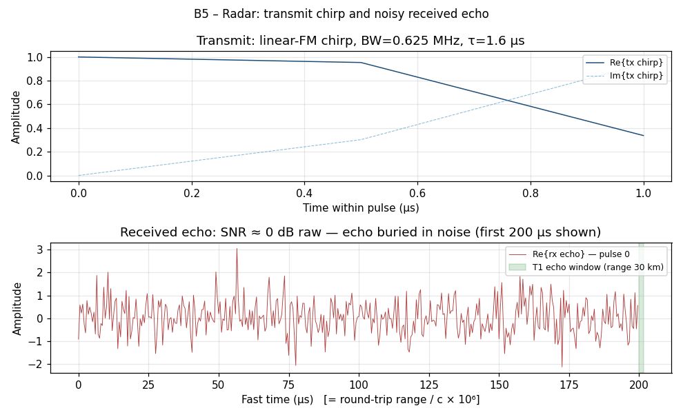
Top: the transmit chirp — frequency sweeps from low to high over
1.6 µs. Bottom: the first 200 µs of the received signal. T1’s echo
(round-trip time 200 µs for 30 km) is completely invisible — buried at 0
dB SNR. The noise floor and the echo have the same amplitude. You cannot
tell by eye that a target is there. Stage 2 will fix that.
Stage
2 — Matched-filter pulse compression: the first Fourier operation
You know exactly what you transmitted. The echo is a delayed,
attenuated, Doppler-shifted copy of it, buried in noise. The optimal
strategy for detecting a known signal in white noise is the
matched filter: cross-correlate the received signal
with the known transmit waveform. In the frequency domain, correlation
is multiplication:
compressed(t) = IFFT( FFT(rx) × conj(FFT(tx)) )That is the entirety of matched-filter pulse compression. The
conj(FFT(tx)) is the matched-filter kernel. Multiply by it
in the frequency domain; IFFT back; T1’s echo emerges as a sharp spike
at the correct range bin.
def matched_filter_compress(raw_matrix, chirp):
    N_FFT   = N_RANGE
    chirp_padded        = np.zeros(N_FFT, dtype=np.complex128)
    chirp_padded[:N_SAMP_PU] = chirp
    TX_CONJ = np.conj(np.fft.fft(chirp_padded))   # matched-filter kernel

    compressed = np.zeros_like(raw_matrix)
    for p in range(N_PULSES):
        RX = np.fft.fft(raw_matrix[:, p], n=N_FFT)
        compressed[:, p] = np.fft.ifft(RX * TX_CONJ).real
    return compressed
Processing gain from coherently integrating N_pulses
= 64 pulses:
SNR_out ≈ SNR_in + 10·log10(N_pulses)
        = 0 dB  + 10·log10(64)
        ≈ 0 dB  + 18 dB
        = 18 dB
The echo that was indistinguishable from noise is now the tallest
feature in the range profile — not because the signal grew stronger, but
because the signal adds coherently across pulses while noise
does not.
Stage 3 —
Doppler DFT: the second Fourier operation
After pulse compression you have a 2D matrix:
compressed[range_bin, pulse_index] # shape: N_range × N_pulses64 columns, one per transmitted pulse. A target at fixed range
appears in the same range bin across all 64 pulses — but its
phase shifts between pulses because the target is
moving. The phase shift per pulse repetition interval (PRI) is:
Δφ = 2π · f_d / PRF, where f_d = 2 · v_r · f_c / cFor each target: – T1 (+20 m/s): f_d = 2 × 20 × 2.8×10⁹ / 3×10⁸ =
373 Hz – T2 (0 m/s): f_d = 0 Hz – T3
(−35 m/s): f_d = −2 × 35 × 2.8×10⁹ / 3×10⁸ = −653
Hz
A DFT across the 64-pulse slow-time dimension of each range bin
converts this phase history to a velocity. That is the Doppler
DFT.
def range_doppler_map(compressed):
    window   = np.hanning(N_PULSES)
    windowed = compressed * window[np.newaxis, :]
    rd_complex = np.fft.fft(windowed, axis=1)        # DFT across slow time
    rd_shifted = np.fft.fftshift(rd_complex, axes=1) # centre zero-Doppler
    return np.abs(rd_shifted)
The Hann window on the slow-time axis suppresses Doppler sidelobes —
same reason you window in audio or vibration analysis. Without it, T2’s
large ground-clutter return at 0 m/s would smear across the whole
velocity axis and mask the precipitation targets.
Stage 4 — The
range-Doppler map: reading the result
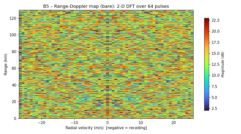
Range-Doppler map. X axis: radial velocity (m/s). Y axis: range
(km). Colour: echo magnitude in dB. Three bright cells at the target
coordinates; everything else is the noise floor. The vertical
zero-Doppler ridge is ground clutter at all ranges.
System resolution for this configuration:
| Metric | Value | Formula |
|---|---|---|
| Range resolution | 240 m | c / (2·BW) |
| Velocity resolution | 84 cm/s | PRF·λ / (2·N_pulses) |
| Unambiguous range | 150 km | c / (2·PRF) |
| Unambiguous velocity | ±26.8 m/s | PRF·λ / 4 |
T3’s true velocity of −35 m/s exceeds the unambiguous velocity of
±26.8 m/s — it folds (velocity aliasing). A real radar uses staggered
PRF or phase-coded pulses to resolve this ambiguity.
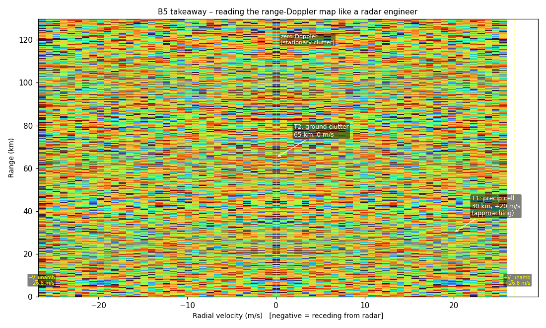
Annotated map. T1: 30 km, +20 m/s (approaching). T2: 65 km, 0 m/s
(stationary clutter). T3: 110 km, aliased from −35 m/s. The unambiguous
velocity boundary (±26.8 m/s) is marked in yellow.
Output SNR after the two Fourier stages (input was 0 dB raw):
| Target | Output SNR |
|---|---|
| T1 (30 km, +20 m/s) | 20.4 dB |
| T2 (65 km, 0 m/s) | 22.2 dB |
| T3 (110 km, −35 m/s) | 17.9 dB |
All three targets detected from a 0 dB raw input. The entire gain —
~20 dB — came from two DFT operations: matched filtering and Doppler
integration.
The
same pattern in your work: cross-domain applications
The radar pipeline — chirp transmit → matched-filter receive
→ Doppler DFT — is not specific to radar. The same mathematical
structure appears wherever you need to detect a known-shape signal in
noise and extract a time delay or a frequency shift.
Ultrasonic distance measurement and NDE. Industrial
ultrasonic gauges and non-destructive evaluation (NDE) systems transmit
a chirp (or tone burst) into a material; the echo is matched-filtered
against the transmitted waveform to locate the back-wall reflection or
an internal flaw with sub-millimetre resolution. The frequency
difference: 40 kHz (air sonar) to 10 MHz (NDE in steel) instead of 2.8
GHz. The mathematics: identical. If you are doing thickness gauging,
weld inspection, or detecting delaminations in composites, this is the
pipeline — and scipy.signal.correlate is the two-line
Python implementation of the matched filter.
Time-domain reflectometry (TDR) for cable fault
location. Inject a chirp or step into a cable; the
matched-filter output on the reflected signal gives you the exact
round-trip time to any impedance discontinuity — a break, a splice, a
corroded connector — with centimetre-level resolution over kilometres of
cable. TDR instruments are radar in a cable. The same range-resolution
formula applies: δ_distance = c / (2·BW·√εᵣ), where εᵣ is the cable
dielectric constant.
Doppler ultrasound (blood flow, fluid flow). Radial
velocity from a moving reflector — blood cells, bubbles in a pipe,
particles in a slurry — via the same f_d = 2·v_r·f_c/c Doppler formula,
at 1–15 MHz carrier instead of GHz. Medical ultrasound machines and
industrial Doppler flow meters both do Stage 3 (Doppler DFT) on each
range gate. Pulse-wave Doppler adds a range gate (Stage 2 matched
filtering) to localise the velocity measurement to a specific depth.
This is the range-Doppler map, inside your hospital’s ultrasound
probe.
Sonar. Active sonar (ship-mounted, towed array,
fish-finder) uses the same three stages at 1–100 kHz in water.
Propagation speed changes (1500 m/s in seawater instead of 3×10⁸ m/s in
air); the mathematics does not.
If any of these appear in your work, the radar chapter is the right
engineering reference — not because you are building radar, but because
you are using the same matched-filter + Doppler-DFT structure that radar
made legible.
When matched filtering
is the right move
You have a signal of known shape buried in noise → matched
filter. If you know what you transmitted (or what you are
looking for), the matched filter is the optimal linear detector for
white noise — by the Schwarz inequality. It maximises the output SNR at
the detection instant. Use it whenever you have a reference waveform:
chirp, tone burst, PN sequence, anything with known structure.
# Generic matched filter via FFT (works for any reference waveform)
signal_spectrum   = np.fft.fft(received, n=N_FFT)
template_spectrum  = np.fft.fft(template, n=N_FFT)
compressed         = np.fft.ifft(signal_spectrum * np.conj(template_spectrum)).real
You have a transient response and want to find exactly when
it arrived → cross-correlation / matched filter. Acoustic echo
timing, impulse response measurement, GPS satellite ranging: all use the
correlation peak to locate the event in time. The FFT-based
implementation is identical to matched-filter compression.
You have a moving target and want to measure velocity →
Doppler DFT. Take multiple snapshots of the same range bin (or
range gate) over time; DFT across the snapshot dimension. The Doppler
frequency bin gives velocity directly via v = f_d · c / (2·f_c). Works
for radar, sonar, ultrasound, and laser Doppler vibrometry equally.
You want both simultaneously → range-Doppler map.
Stack the matched-filter output (range axis) and slow-time DFT (velocity
axis) into a 2D image. This is the structure of every coherent
pulse-Doppler instrument, from weather radar to medical pulsed-wave
Doppler.
Pitfalls to know before
you implement
Nyquist applies to the highest frequency in your chirp, not
just the carrier. If your chirp sweeps from f_c to f_c + BW,
your ADC must sample at ≥ 2·BW after down-conversion to baseband (or ≥
2·(f_c + BW) if you are sampling the RF directly). In the simulation:
f_s = 2 MHz = 2 × BW = 2 × 0.625 MHz — exactly at Nyquist. In practice,
add margin (2.5–3× BW is common for anti-alias filter roll-off).
PRF controls two ambiguity boundaries that trade against each
other. Higher PRF → better unambiguous velocity (±PRF·λ/4) but
shorter unambiguous range (c/(2·PRF)). This simulation: PRF gives 150 km
unambiguous range and ±26.8 m/s unambiguous velocity — T3 at −35 m/s
folds. For the same λ, you cannot extend both simultaneously without
staggered PRF or waveform coding.
Doppler frequency resolution depends on integration time, not
on BW. Velocity resolution = PRF·λ/(2·N_pulses). You improve it
by integrating more pulses (longer coherent processing interval), not by
increasing BW. BW buys range resolution; integration time buys velocity
resolution. The two are independent — this is the radar analogue of the
time-bandwidth product in communications.
Practitioner takeaway
The three-stage pipeline is:
1. Chirp (known waveform) → encodes range in time delay
2. Matched filter (FFT × conj(FFT) → IFFT) → extracts range, converts 0 dB SNR to ~18 dB
3. Doppler DFT (FFT across slow time) → extracts velocity from phase history
The DFT is doing structural work in all three stages — not just
describing a spectrum, but solving for a physical quantity. That is what
“spectrum as measurement” means.
If your engineering problem involves detecting a known waveform in
noise, locating an echo in time, or extracting velocity from phase shift
— this pipeline is what you are implementing, whether or not the word
“radar” appears anywhere in your job description.
Go deeper
Full engineering treatment — derivations, complete code, all system
parameters:
→ lege-artis/fourier/docs/shad/05-radar.md
Runnable simulation (NEXRAD-analogue; generates all three
figures):
→ lege-artis/fourier/examples/shad/b5-radar/main.py
git clone https://github.com/lege-artis/fourier.git
cd fourier/examples/shad/b5-radar
pip install numpy matplotlib
python main.py
The broader guide — from DFT foundations (B0–B1) through vibration
diagnostics (B3), this radar capstone (B5), and beyond-Fourier methods
(B7) — is at lege-artis/fourier.
References
-
M. Skolnik, Introduction to Radar Systems, 3rd ed.,
McGraw-Hill (2001). Ch. 8 (pulse compression), Ch. 3 (Doppler
processing). (The practitioner’s standard radar reference;
matched-filter derivation in §8.2.) -
M. Richards, J. Scheer, W. Holm (eds.), Principles of Modern
Radar: Basic Principles, SciTech Publishing (2010). Ch. 17
(range-Doppler processing). (More mathematically precise on the
signal-processing side.) -
NOAA, Doppler Radar Meteorological Observations, Federal
Meteorological Handbook No. 11, Part B (2005). (Operational WSR-88D
NEXRAD documentation; the system this simulation is modelled
on.)