From Signal to Spectrum: What an Oscilloscope Cannot Tell You
You have a scope. You have a trace. You can see something oscillating, or decaying, or ringing. The scope shows you voltage over time — and that is genuinely useful. But it is also, in almost every interesting case, the wrong picture. This post shows you the right one.
What you need to follow along
Hardware + software checklist
To replicate the examples in this post you need:
Python 3.9+ with NumPy and Matplotlib:
pip install numpy matplotlib scipyThe lege-artis/fourier example scripts (optional but recommended — they generate the exact signals used here):
git clone https://github.com/lege-artis/fourier.git
cd fourier/examples/shad/b1-scope
A scope with USB/CSV export (optional) — any modern DSO that can save a CSV of its trace, whether a Rigol, Siglent, or Tektronix, will plug directly into the pipeline below. You do not need one to follow this post; all four signals are analytically generated or fetched from public datasets.
The bar for hands-on engagement is low. If you can run Python, you can replicate every spectrum in this post from scratch.
What the DFT actually does, in two hundred words
The Discrete Fourier Transform is a machine with a specific I/O contract. You give it N equally-spaced samples of a signal. It gives you back N complex numbers — one per frequency bin. Each complex number encodes the amplitude and phase of one sinusoidal component at the corresponding frequency. You take the magnitude with np.abs() and you have the spectrum: a bar chart of “how much of each frequency is present.”
import numpy as np

spec = np.fft.fft(x)        # x is your N-sample array
freq = np.fft.fftfreq(N, d=dt)  # dt = sample spacing in seconds
mag  = np.abs(spec[:N//2])  # one-sided magnitude spectrum
That is the whole pipeline. Three lines of Python.
The bin spacing — the frequency resolution — is 1 / (N × dt), i.e. the reciprocal of the total observation window. A 100 ms capture at 50 kHz gives you bins spaced 10 Hz apart. A 1 s capture gives you 1 Hz bins. You get better frequency resolution by capturing longer, not by sampling faster.
The highest frequency the DFT can represent is the Nyquist frequency: half the sample rate. At 50 kHz sample rate, the spectrum runs from 0 Hz to 25 kHz. Any signal above 25 kHz will alias — appear at a lower frequency than it actually occupies. This is a hard limit, not a suggestion.
Now apply it to four real signals.
Fixture 1 — Radioactive decay
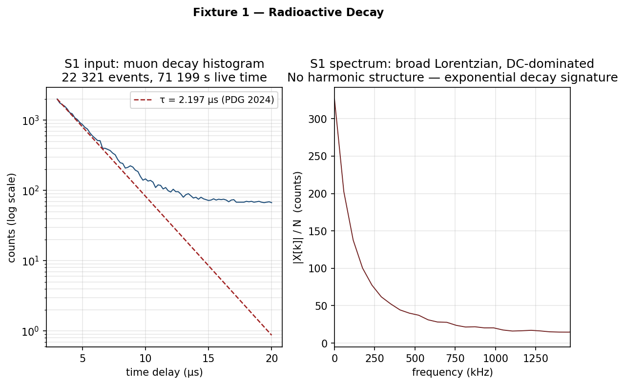
Left: muon-lifetime histogram — 22 321 decay events accumulated over 71 199 s of live time, rebinned to 0.2 µs per bin. Right: one-sided DFT magnitude. DC-dominated, with a broad Lorentzian rolloff and no harmonic structure.
What generated this signal
A muon telescope at a university physics lab. Cosmic-ray muons stop in a scintillator detector; a multi-channel analyser (MCA) records the time between the stop signal and the subsequent decay signal. The MCA is, in effect, a stopwatch: it bins events into 16 384 channels each 2.3 nanoseconds wide, running a time calibration of t_ns = 2.2986 × channel − 162.8.
A muon decays into an electron and two neutrinos with a mean life of τ ≈ 2.197 µs (PDG 2024). The histogram is therefore an exponential decay: count(t) ∝ exp(−t/τ), with a flat background at late times from accidental coincidences.
The dataset — 22 321 muon decays accumulated over 71 199 s of live time — is the Rodriguez MCA dataset, available at amor.cms.hu-berlin.de/~rodrigus under Santiago Rodriguez’s copyright (cite key Rodriguez2018; public redistribution requires written permission).
The spectrum
The Fourier transform of an exponential decay is a Lorentzian: a broad, smooth hump centred at DC. There are no peaks, no harmonics, no periodic structure. The muon does not ring. It decays at a random time with a known average — the spectrum reflects that statistical randomness as spectral broadness.
What the DFT tells you that the scope cannot: the shape of the spectrum alone distinguishes “random exponential decay” from “periodic signal.” No model fitting, no eye-balling the decay constant — the spectrum is unambiguous. The flat background of accidentals contributes a flat floor across all frequency bins, separately visible and separately interpretable.
Fixture 2 — 1 kHz square wave

Left: first 5 ms of the square wave — sharp transitions at each half-period. Right: DFT magnitude on a log scale. Peaks appear only at odd harmonics: 1, 3, 5, 7, 9 kHz.
What generated this signal
A function generator output: sign(sin(2π·f·t)) with f = 1 kHz. Sample rate 50 kHz, duration 100 ms, 5000 samples. This is the mathematical definition of a square wave — the waveform a digital clock line drives, or what a Rigol DG1022 puts on the scope screen when you ask it for a square.
The spectrum
Run the three-line DFT pipeline and you get a sparse comb:
k=100  f=1000 Hz  |X|=0.6366   (expected 2/π = 0.6366) ✓
k=300  f=3000 Hz  |X|=0.2121   (expected 2/3π = 0.2122) ✓
k=500  f=5000 Hz  |X|=0.1272   (expected 2/5π = 0.1273) ✓
k=700  f=7000 Hz  |X|=0.0908   (expected 2/7π = 0.0909) ✓
Odd harmonics only; even harmonics are exactly zero. Amplitudes follow 2/(πn) for harmonic n = 1, 3, 5, … — the Fourier series result that Joseph Fourier computed in 1822. The DFT matches his prediction to four decimal places, two centuries later, on a laptop.
On a log scale the peaks fall in a perfect straight line — the 1/n amplitude envelope plotted logarithmically.
What this means for your circuit
The “simple” digital square wave contains an infinite harmonic series. Any bandlimited channel — a transmission line, a PCB trace, a filter — will clip the high harmonics. A 1 Mbps clock carries significant Fourier energy out to 5 MHz, 10 MHz, and beyond. Clip that energy, and the transitions that distinguish a 1 from a 0 degrade. The spectrum shows you exactly where the energy lives and what bandwidth your channel needs to reproduce the waveform faithfully.
What the DFT tells you that the scope cannot: the scope shows you “sharp transitions.” The DFT shows you exactly which harmonics exist and at what amplitude — the full frequency budget of the waveform.
Try it yourself
import numpy as np
import matplotlib.pyplot as plt

fs = 50_000      # Hz
T  = 0.1         # seconds
N  = int(fs * T) # 5000 samples
t  = np.arange(N) / fs

v    = np.sign(np.sin(2 * np.pi * 1000 * t))   # 1 kHz square
spec = np.fft.fft(v) / N
freq = np.fft.fftfreq(N, d=1.0/fs)
half = N // 2
mag  = np.abs(spec[:half])

plt.semilogy(freq[:half], mag)
plt.xlabel("frequency (Hz)"); plt.ylabel("|X[k]| / N")
plt.title("1 kHz square wave — odd harmonic comb")
plt.show()
Run this and you reproduce the spectrum above. Change 1000 to 1500 and the entire harmonic comb shifts in lockstep. Change np.sign(...) to (2/np.pi) * np.arcsin(np.sin(...)) and the comb stays at the same positions but the amplitudes switch from the 1/n to the 1/n² envelope — Fixture 3.
Fixture 3 — 1 kHz triangle wave

Left: first 5 ms — same frequency as the square wave, visibly smoother. Right: DFT magnitude spectrum overlaid with the square wave spectrum from Fixture 2. Same harmonic positions; different amplitudes.
What generated this signal
Same function generator, same parameters: (2/π)·arcsin(sin(2π·f·t)) — the mathematical triangle wave. Sample rate 50 kHz, 100 ms, 5000 samples. Same frequency, same amplitude, different shape.
The spectrum
The harmonic series is identical in structure to the square wave — odd harmonics only, at 1, 3, 5, 7 kHz. The difference is the amplitude envelope:
              Square (S2)          Triangle (S3)
Fundamental:  2/π   = 0.6366      4/π²  = 0.4050
3rd harmonic: 2/3π  = 0.2121      4/9π² = 0.0449    (9× smaller than S3 fund.)
5th harmonic: 2/5π  = 0.1273      4/25π²= 0.0162    (25× smaller)
7th harmonic: 2/7π  = 0.0909      4/49π²= 0.0083
The square wave has a 1/n envelope; the triangle wave has a 1/n² envelope. Harmonics fall much faster. The third harmonic of the triangle wave is fourteen times smaller relative to its fundamental than the corresponding harmonic of the square wave.
This is why a triangle wave sounds softer than a square wave at the same frequency. It is also why triangle-wave oscillators are used in analog synthesizers when you want a less harsh timbre than a square — you are choosing a different spectral shape, not just a different waveform shape.
What the DFT tells you that the scope cannot: two signals at the same frequency, both “periodic,” look superficially similar on the scope (both symmetric, both regular). The DFT separates them unambiguously: the harmonic falloff rate is the fingerprint.
Fixture 4 — RLC damped transient
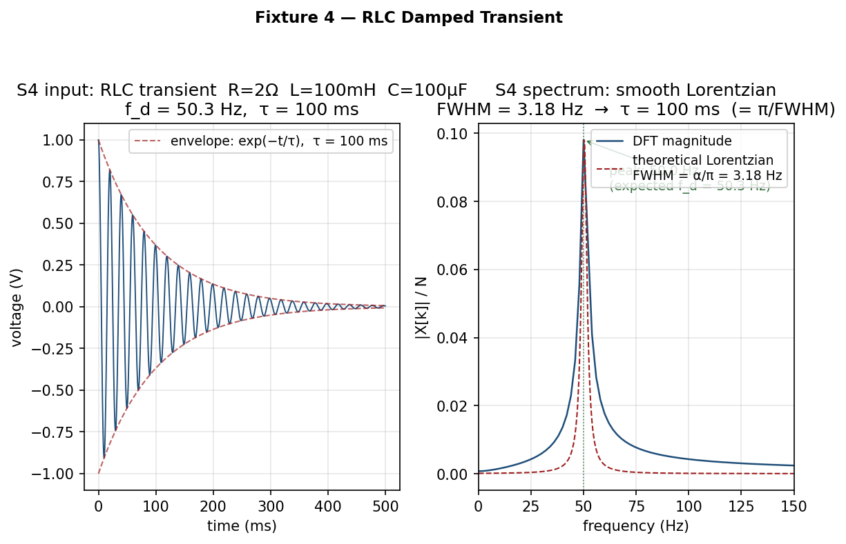
Left: capacitor voltage after a step input — the decay envelope exp(−t/τ) with τ = 100 ms is clearly visible. Right: DFT magnitude spectrum — a smooth Lorentzian centred near 50 Hz.
What generated this signal
The step response of an underdamped series RLC circuit: R = 2 Ω, L = 100 mH, C = 100 µF. After a voltage step at t = 0, the capacitor voltage rings at the damped resonance frequency:
v(t) = exp(−α·t) · cos(ω_d·t)
  where  α     = R/(2L)           = 10.0 rad/s  →  τ  = 100 ms
         ω_0   = 1/√(LC)          = 316.2 rad/s →  f_0 = 50.3 Hz
         ω_d   = √(ω_0² − α²)    ≈ 316.0 rad/s →  f_d = 50.3 Hz
Sample rate 2 kHz, duration 500 ms, 1000 samples. This is the signal you see when you probe across the capacitor of an underdamped RLC circuit after flipping the input.
The spectrum
A smooth hump centred near 50 Hz. Not a sharp spike — a broad Lorentzian, the Fourier transform of an exponential decay:
|X(f)|² ∝ 1 / [(f − f_d)² + (α/2π)²]The half-power (−3 dB) width of the hump is α/π:
Peak: 50.00 Hz  (expected f_d = 50.30 Hz; 2 Hz = 1 bin at fs=2 kHz, N=1000)
FWHM: 3.18 Hz   (= α/π = 10/π)
tau : 100 ms    (= π/FWHM = 1/α)
Here is the key insight: the spectral width and the decay time are the same measurement in two different domains. A circuit that rings for a long time (small α) has a narrow spectral peak — it is “tone-like.” A circuit that damps out quickly has a broad, fat spectral hump. The relationship FWHM = α/π = 1/(π × τ) is exact. You can read the time constant off the frequency-domain picture without touching the time-domain envelope.
What the DFT tells you that the scope cannot: the scope shows you “ringing.” The DFT tells you the resonant frequency and the damping constant simultaneously, from a single spectrum. This generalises to any damped resonance — structural vibration, acoustic resonance, resonant cavity, bearing fault — wherever a system rings at a characteristic frequency and decays.
Engineering applications of the Lorentzian width
The FWHM = 1/(π·τ) relationship is more powerful than it might look. In vibration diagnostics you hit a structure with an impulse hammer and record the ring-down; the spectral peak width tells you the mechanical damping without requiring a curve fit to the time-domain envelope. In RF engineering the spectral width of an oscillator’s output tells you its phase noise and settling time. In bearing-fault analysis a worn bearing produces a periodic impulse train at the defect frequency, visible as a harmonic comb — but the width of each harmonic tells you whether the defect is sharp (localised damage) or diffuse (general wear).
The scope shows you time. The spectrum shows you physics.
Common pitfalls
Three things bite practitioners who are new to the DFT. None of them require mathematics to understand.
Spectral leakage
If the signal you are transforming is not an integer number of complete cycles within your observation window, the DFT smears energy from the true frequency into adjacent bins. A 1 kHz tone sampled for 99 ms (99 complete cycles) is fine. A 1 kHz tone sampled for 99.5 ms — not an exact number of periods — will show leakage: a strong peak at 1 kHz with visible sidebands spreading to adjacent bins.
The fix is windowing: multiply the time-series by a window function (Hann, Blackman-Harris, flat-top) that tapers to zero at both ends before transforming. This trades a small amount of frequency resolution for a dramatic reduction in sidelobes.

Left: rectangular window (no windowing) — energy from a non-integer-period tone spreads into adjacent bins. Right: Hann window applied — the same tone resolves to a clean, well-localised peak.
Nyquist aliasing
Any spectral content above half the sample rate will appear at the wrong frequency in your spectrum. A 30 kHz tone present in a signal sampled at 44.1 kHz shows up at 44100 − 30000 = 14.1 kHz — completely misleading. Add an anti-aliasing filter before your ADC if signal content above Nyquist is physically possible.
Bin spacing ≠ frequency resolution
The bin spacing Δf = 1/(N × dt) tells you how far apart the DFT samples the frequency axis. Frequency resolution — the minimum separation between two tones you can distinguish — is determined by the window function and is typically 1–2× the bin spacing for rectangular windows, and 2–4× for tapered windows. Increasing sample rate does not improve frequency resolution; only increasing observation duration does. A common mistake is to zoom in on the spectrum and conclude that two tones 5 Hz apart are “clearly resolved” because they land in adjacent bins — then discover that a different windowing choice merges them into a single broad peak. Always check with the window you will actually use in production.
When to reach for this tool
Reach for the DFT when:
You have a time-series and suspect periodicity. Vibration logs, power-quality measurements, biological signals, mechanical wear indicators — anything that might repeat. The DFT converts “does this signal repeat?” from a visual inspection problem into a peak-finding problem.
You have a noise problem and want to locate it in frequency. Switching noise at 100 kHz, mains hum at 50/60 Hz, RF interference at a known carrier frequency — these all show up as identifiable peaks in the spectrum. Once you see where the noise lives, you know what filter to build.
You have a physical system and want to characterise its resonances. Hit a mechanical structure, an acoustic cavity, or an electrical circuit with a broadband impulse (a step, a click, a hammer tap) and transform the ring-down. The spectral peaks are the natural modes; their widths are the damping constants. This is frequency-response measurement without a network analyser.
Do not reach for the DFT when:
The timing of a short transient matters more than its frequency content. If you need to know when something happened — a glitch, a pre-breakdown discharge, the exact moment of mechanical impact — the DFT will smear that information across the spectrum. The DFT trades time localisation for frequency resolution. For short-duration transients where both matter, the right tool is the wavelet transform, which provides simultaneous time-frequency localisation at the cost of a more complex interpretation framework.
What to read next
The post you are reading is the entry point. The engineering-grade reference — with runnable Python for all four fixtures, the derivation of the Lorentzian width formula, and worked examples covering seven domains from oscilloscope to radar to nuclear reactor noise — is the lege-artis/fourier repository:
- B1 chapter (this post, extended):
fourier/docs/shad/01-oscilloscope.md - Runnable example scripts:
fourier/examples/shad/b1-scope/ - Full seven-domain guide:
lege-artis/fourier
The next natural step after this post is B5 — Radar: the chapter where the spectrum itself becomes the measurement, and the DFT extracts distance and velocity from echo timing. It is the same three lines of code, applied to a domain where the physical interpretation is completely different.
The four fixtures, summarised
| Signal | Time domain | Frequency domain | Key number |
|---|---|---|---|
| S1 — muon decay | Exponential decay + flat background | Broad Lorentzian, DC-dominated, no harmonics | τ = 2.197 µs |
| S2 — square wave | Sharp periodic transitions | Sparse odd-harmonic comb, 1/n amplitude envelope | 2/π = 0.6366 at fundamental |
| S3 — triangle wave | Smooth periodic ramps | Same odd harmonics, 1/n² envelope | 4/π² = 0.4050 at fundamental |
| S4 — RLC transient | Decaying oscillation | Smooth Lorentzian, FWHM = α/π | FWHM = 3.18 Hz; τ = 100 ms |
The DFT does not know it is looking at a physics experiment in one case, a function generator in two, and a passive circuit in another. It asks the same question of all four: at what frequencies, and with what amplitude, does this signal repeat? The answer is different every time. The question — and the three lines of code — are always the same.
References
-
S. Rodriguez, Muon Lifetime Data, 2018–2022. Available at
amor.cms.hu-berlin.de/~rodrigus. © 2018–2022 Santiago Rodriguez. Cite keyRodriguez2018. (Fixture 1 source data; public redistribution requires written permission.) -
J. B. J. Fourier, Théorie analytique de la chaleur, Paris, 1822. (The odd-harmonic series for square and triangle waves is a direct consequence of the Fourier coefficients computed here. Fourier himself was working on heat propagation; the application to scope traces would have surprised him only in the matter of the scope.)
-
Particle Data Group, R. L. Workman et al., Review of Particle Physics, PTEP 2022 (2022) 083C01. Muon mean life: τ = 2.1969811 µs ± 0.0000022 µs.